Excel Conditional Formatting Based On Another Cell

Are you ready to unleash the power of Excel and take your spreadsheet game to the next level? One of the most exciting features in Excel is Conditional Formatting, which allows you to highlight cells based on specific conditions. But what makes it even more useful is when you can format cells based on another cell's value!

The purpose of this feature is to help you visualize and analyze your data more efficiently. By highlighting cells based on another cell's value, you can quickly identify trends, patterns, and correlations. The benefits are numerous, including improved decision-making, enhanced data insight, and increased productivity.

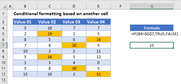
For example, imagine you have a spreadsheet with sales data, and you want to highlight cells where the sales amount exceeds a certain threshold. You can use Conditional Formatting to achieve this. Or, suppose you have a list of tasks with deadlines, and you want to highlight tasks that are due soon. With Excel, you can format cells based on another cell's value, making it easy to prioritize and manage your tasks.

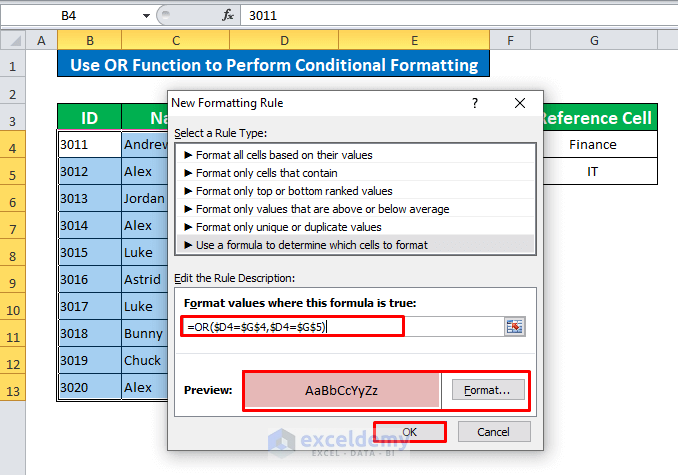
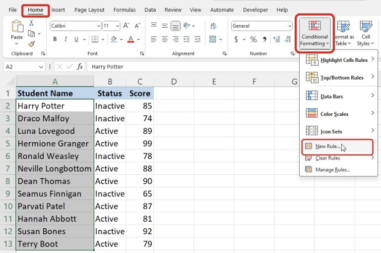
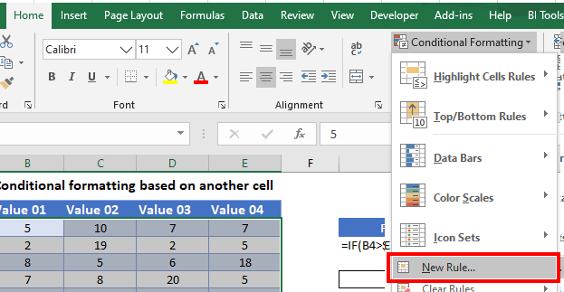
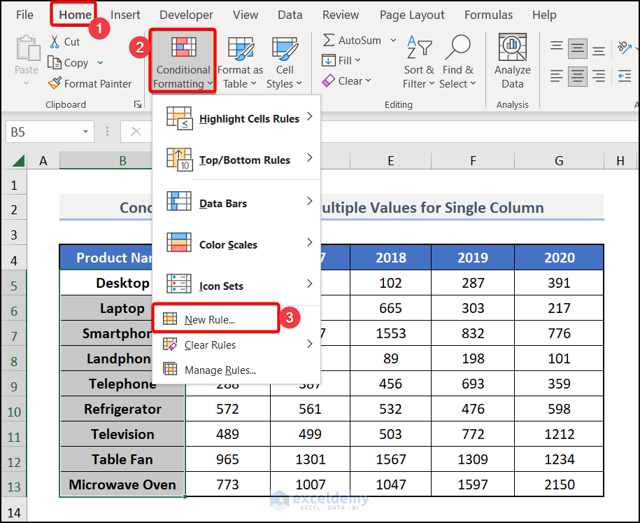
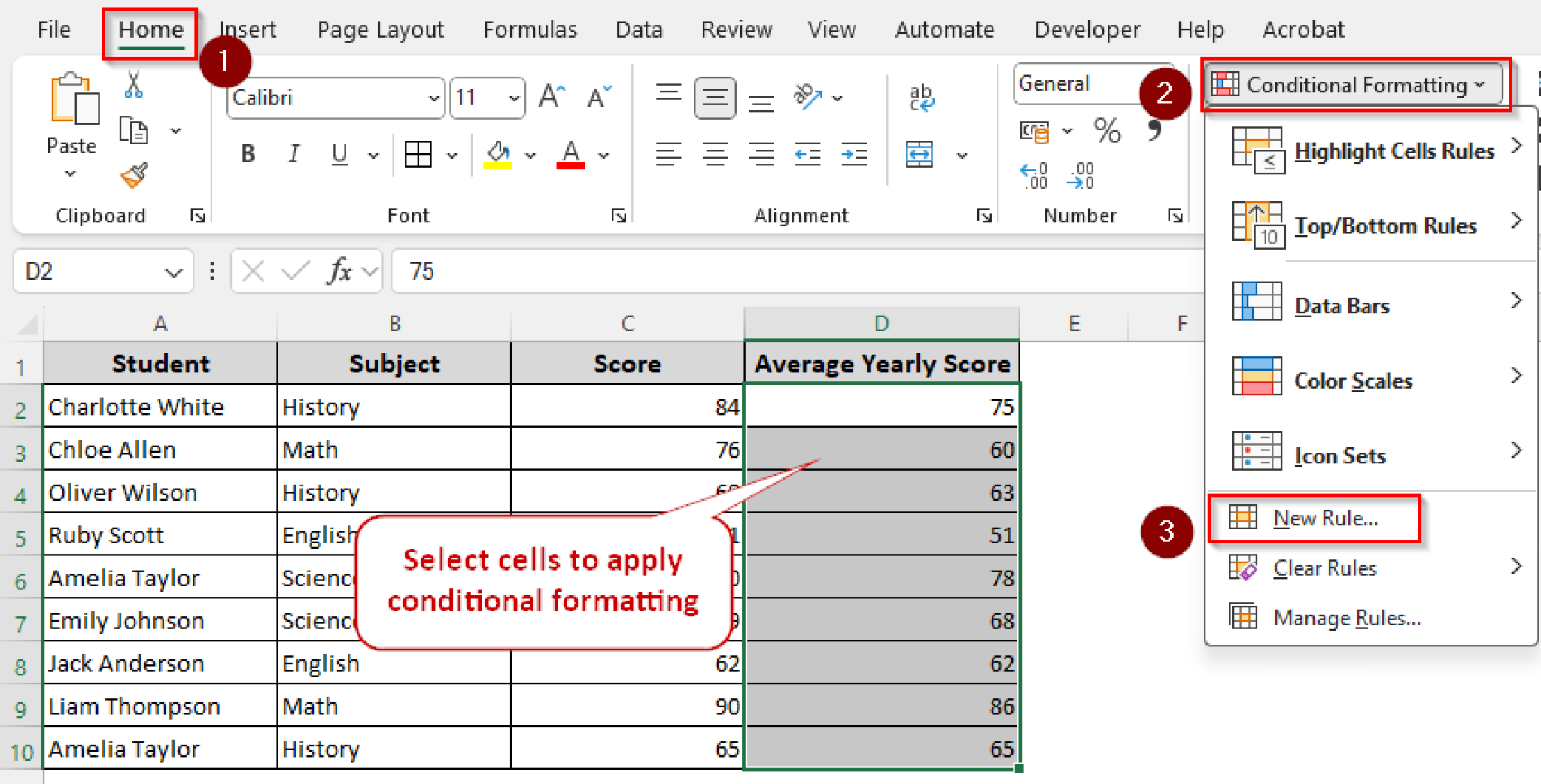
Here's a practical tip: to use Conditional Formatting based on another cell, select the cell range you want to format, go to the Home tab, click on Conditional Formatting, and then choose "New Rule". From there, you can specify the condition based on another cell's value. With this feature, the possibilities are endless, and you'll be amazed at how much more efficient and effective you can be with your Excel spreadsheets!