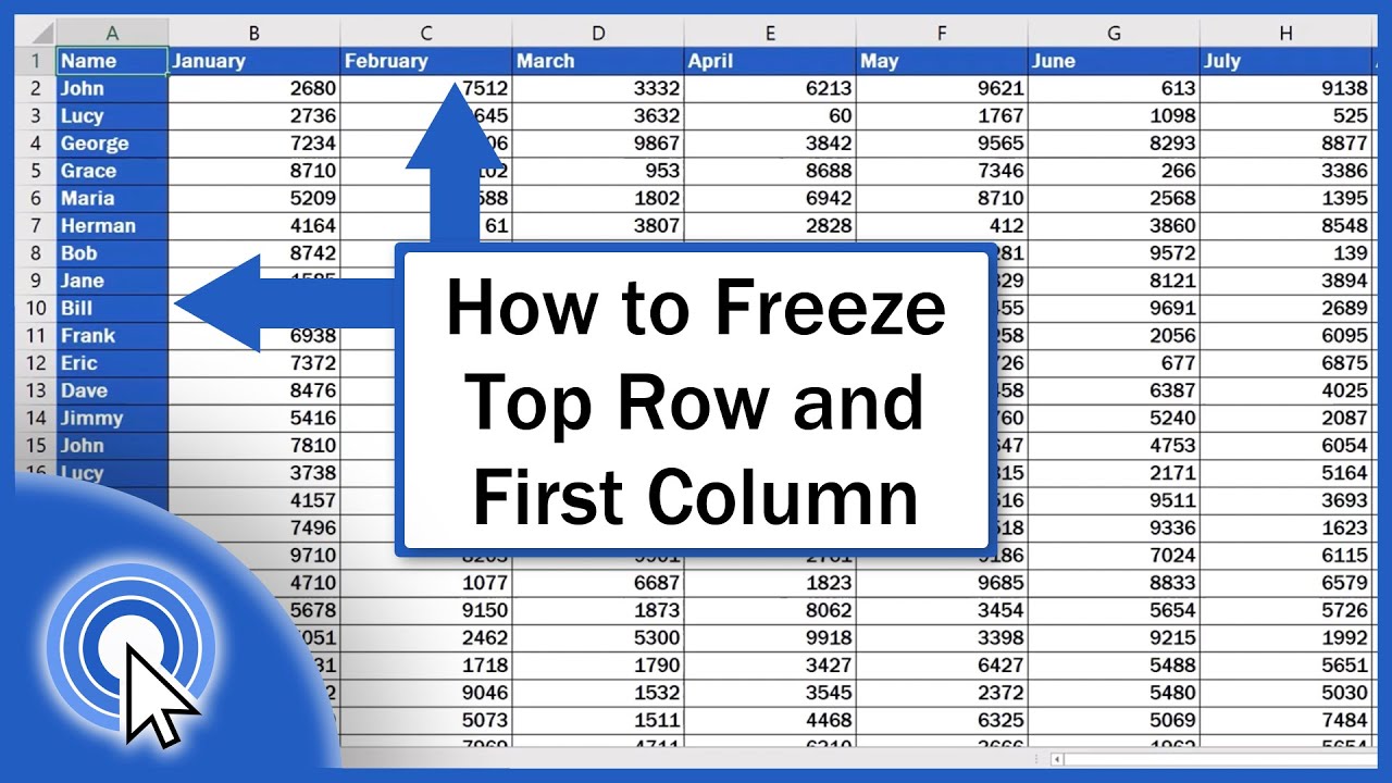
See How To Freeze Top Row And First Column In Excel For Free
Working with large datasets in Excel can be overwhelming, especially when you need to reference specific headers or columns repeatedly. That's where freezing panes comes in - a game-changer for anyone who uses Excel regularly. Whether you're a beginner looking to improve your spreadsheet skills or a hobbyist trying to organize your personal finances, freezing the top row and first column can be a huge time-saver.
The purpose of freezing panes is to lock specific rows or columns in place, making it easier to navigate and reference your data. This is particularly useful for families who need to track budgets or schedules, as well as students working on projects that involve large datasets. By freezing the top row and first column, you can quickly identify headers and categories, even when scrolling through hundreds of rows.
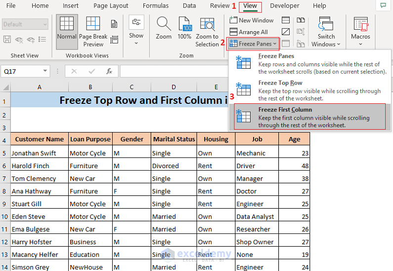
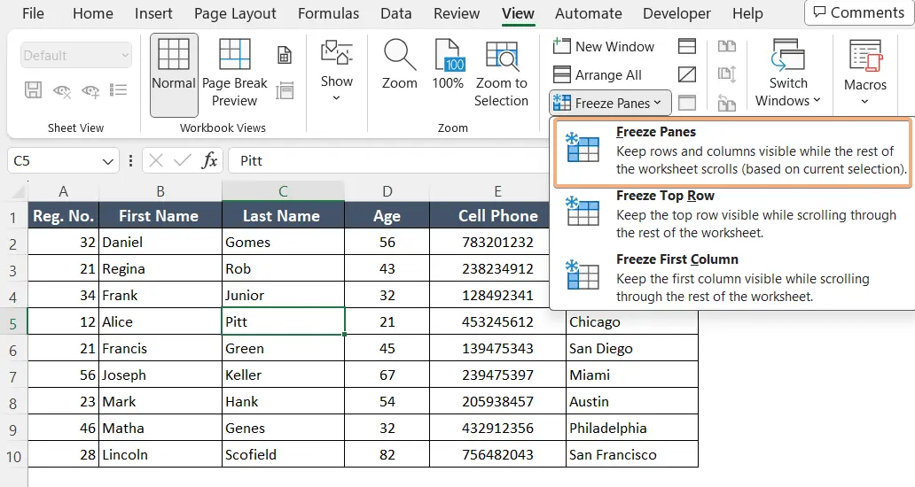
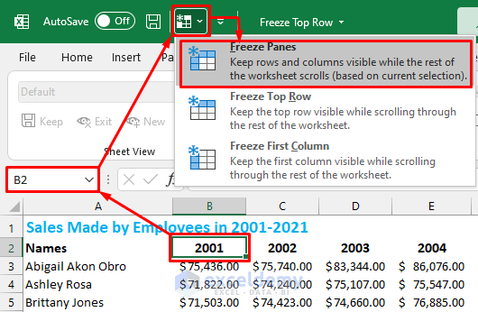
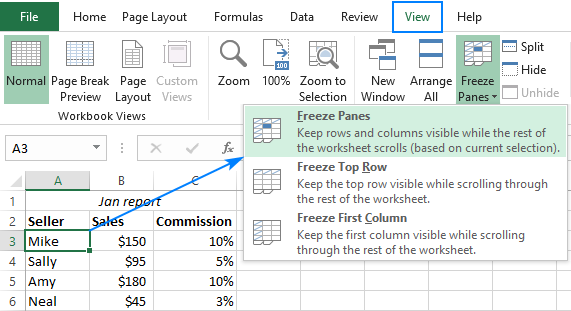
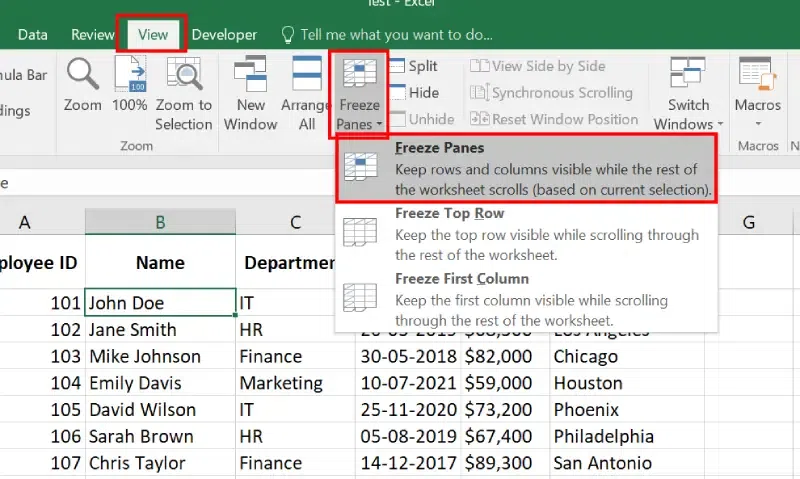
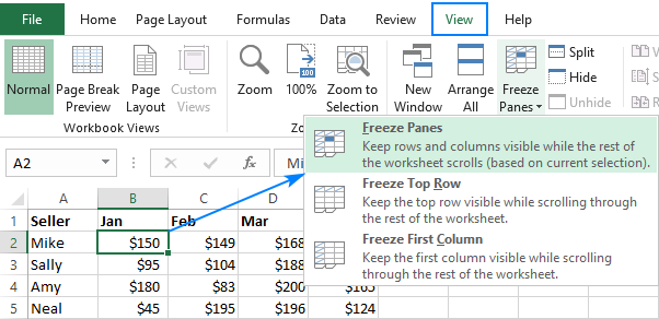
To get started, simply select the cell below the row you want to freeze and to the right of the column you want to freeze, then go to the View tab and click on Freeze Panes. You can also use the shortcut keys Alt + W + F to freeze panes quickly. With this simple trick, you can boost your productivity and make working with Excel a breeze.
Must Read
In conclusion, freezing the top row and first column in Excel is a simple yet powerful technique that can benefit anyone who uses the software. By following these easy steps, you can transform your workflow and make data analysis a whole lot easier. So why not give it a try and see the difference for yourself?